Table of Contents
The Evolution of Rule-Based Monetary Policy and the Taylor Principle
The conceptualization of monetary policy as a systematic, rule-governed endeavor fundamentally transformed the landscape of central banking in the late 20th century. Historically, the discourse surrounding whether monetary policy should be based on intuition and discretion or guided by a formal rule began as early as the 19th century. However, it was not until John B. Taylor’s seminal 1993 paper that a simple, prescriptive equation gained widespread acceptance as a benchmark for the federal funds rate. The Taylor rule relates the short-term interest rate targeted by the Federal Open Market Committee (FOMC) to the current state of inflation and economic slack, typically measured as the output gap or unemployment gap.
At its core, the original Taylor rule posits that for every percentage point increase in inflation above the target, the central bank should raise the nominal interest rate by more than one percentage point. This specific response, known as the Taylor principle, ensures that the real interest rate increases in response to rising inflation, thereby providing a stabilizing counter-cyclical mechanism. In the “textbook” New Keynesian model, satisfying the Taylor principle is considered both a necessary and sufficient condition for stabilizing inflation expectations. When the Taylor principle is violated, the real interest rate remains unchanged or falls as inflation rises, which can lead to self-fulfilling economic fluctuations and “sunspot” equilibria where inflation becomes indeterminate and potentially explosive.
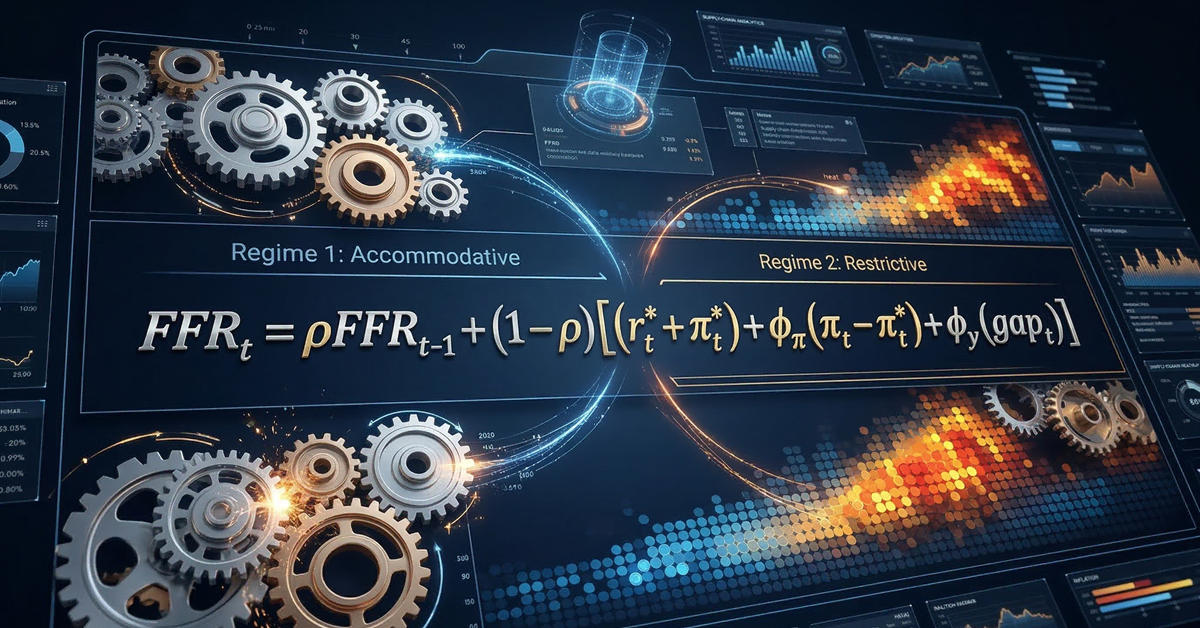
The mathematical foundation of the rule is generally expressed as:
In this framework, is the prescribed policy rate, is the natural or equilibrium real interest rate, is the target inflation rate, and represents the deviation of actual output from potential. The coefficient accounts for interest rate smoothing, reflecting the tendency of central banks to adjust rates in small, incremental steps rather than large, abrupt shifts.
| Taylor Rule Element | Theoretical Value | Empirical Variation | Significance |
| Inflation Coefficient () | 1.5 | 0.8 to 4.0 | Determines adherence to the Taylor Principle |
| Output Gap Coefficient () | 0.5 | 0.0 to 2.0 | Reflects the weight on the employment mandate |
| Smoothing Parameter () | 0.0 | 0.7 to 0.9 | Accounts for gradualism in policy moves |
| Inflation Target () | 2.0% | 1.5% to 4.0% | Anchors long-run price expectations |
| Natural Rate () | 2.0% | -1.0% to 3.0% | Defines the neutral policy stance |
Theoretical Foundations of Markov-Switching in Econometrics
While the original Taylor rule provided an exceptionally good fit for U.S. monetary policy during the “Great Moderation” (roughly 1987 to 2006), its descriptive power has been found to be fragile across different economic eras. Standard linear models with constant coefficients fail to capture the reality that central bankers may change their policy weights or objectives in response to structural changes in the economy, shifts in political pressure, or the emergence of unprecedented shocks. To address this, researchers utilize Markov-switching (MS) models, which characterize data as falling into different, recurring “regimes” or “states”.
In a Markov-switching Taylor rule, the parameters—including the response to inflation, the response to the output gap, and the variance of the policy shocks—are allowed to vary across unobserved states governed by a stochastic process. The transition between these states is determined by a Markov chain, where the probability of being in a certain state today depends only on the state of the previous period. This allows the econometric model to distinguish between “hawkish” regimes, where the Taylor principle is strictly followed, and “dovish” or “passive” regimes, where the central bank may prioritize output management or financial stability at the expense of inflation targeting.
The appeal of MS models in monetary analysis lies in their ability to endogenously identify regime transitions without requiring the researcher to exogenously specify dates for structural breaks. This is particularly relevant for analyzing the tenure of Federal Reserve Chairs like Paul Volcker; while traditional accounts suggest a single “Volcker revolution,” MS analysis reveals a more complex picture of shifting regimes within his tenure, including periods where the Taylor principle was actually violated as the Fed experimented with non-borrowed reserve targeting.
Mechanics of State Transition and Estimation
The complete Markov-switching model involves an assumed number of regimes (typically two or three), independent variables (inflation and output gap), and transition probabilities that describe the likelihood of a regime shift. Estimation is generally conducted using either Maximum Likelihood Estimation (MLE) via the Expectation-Maximization (EM) algorithm or Bayesian estimation using Markov Chain Monte Carlo (MCMC) methods such as Gibbs sampling.
The EM algorithm, first proposed by John Hamilton in 1990, iteratively estimates the latent variable (the E-step) and then the parameters of the model (the M-step) until convergence. Bayesian methods, conversely, rely on drawing samples from the joint distribution of parameters and states, which is particularly useful when the likelihood function is complex or when incorporating prior beliefs about central bank behavior. These techniques allow researchers to identify time-varying persistence and uncertainty in the inflation process, confirming that inflation often switches from a low-variance regime with a stable mean to a high-variance, random-walk regime during periods of economic turbulence.
Historical Regime Analysis: From Great Inflation to Great Moderation
The application of Markov-switching models to U.S. data over the past sixty years reveals several distinct eras of monetary policy behavior. The period from 1965 to 1979, known as the “Great Inflation,” is frequently identified as a regime where the Taylor principle was systematically violated. During this era, the coefficient on inflation was often significantly less than one, meaning the Federal Reserve did not raise nominal interest rates enough to increase the real interest rate in response to rising prices. This lack of aggressive response is cited as a primary driver for the unanchoring of inflation expectations and the transition of inflation into a non-stationary process.
A common finding in MS literature is that the Fed consistently adhered to the Taylor principle before 1973 and after 1984, but the intervening decade was marked by significant regime instability. Interestingly, some models identify a “dove regime” that accommodates increases in the natural rate of unemployment and a “hawk regime” that reacts strongly to inflation deviations. The Volcker tenure (1979-1987) is often modeled as a transition period; while it is popularly viewed as a hawk regime, MS analysis shows that the Fed did not strictly follow a standard interest-rate rule during the initial disinflationary push, instead focusing on monetary aggregates, which resulted in “positive deviations” where the actual funds rate was far higher than a Taylor rule would have prescribed.
The Great Moderation and the “Mythical Status” of the Taylor Rule
The period starting in 1987, under the leadership of Alan Greenspan, is widely regarded as the era when the Taylor rule was most descriptive of actual policy. During this time, the Fed maintained a consistent regime of inflation targeting and output stabilization, leading many economists to view the Taylor rule as virtually synonymous with good monetary policy. However, even during this stable era, researchers have noted that the Fed may have implicitly shifted its weights. Janet Yellen, for instance, suggested that a “balanced approach” would imply a coefficient of 1.0 on the output gap rather than Taylor’s original 0.5.
| Era Name | Approximate Dates | Adherence to Taylor Principle | Dominant Objective |
| Great Inflation | 1965 – 1979 | No (Violation) | Output Gap / Employment |
| Volcker Transition | 1980 – 1985 | Inconsistent/Non-linear | Inflation (via aggregates) |
| Great Moderation | 1987 – 2000 | Yes (Consistent) | Balanced Dual Mandate |
| Post-Dotcom | 2001 – 2007 | Yes (Low Deviations) | Stability / Growth |
| GFC & ZLB | 2008 – 2015 | No (Censored at 0) | Financial Solvency / Recovery |
| Post-COVID | 2021 – 2024 | Delayed / Asymmetric | “Looking Through” Shocks |
Supply Shocks and the “Targeted Taylor Rule” Framework
A critical limitation of the standard Taylor rule is its “one-size-fits-all” response to inflation, regardless of the underlying driver. Monetary theory prescribes a forceful reaction to demand-driven inflation, where inflation and output move in the same direction, but an attenuated response to supply-driven (cost-push) inflation, where inflation rises while output and employment fall. If a central bank reacts too aggressively to a supply shock, it risks amplifying the decline in employment—a trade-off that has become central to recent policy deliberations.
Recent research from the Bank for International Settlements (BIS) and other institutions has introduced the concept of a “targeted Taylor rule,” which decomposes inflation into its demand- and supply-driven components. Empirical estimations for the United States since the Volcker era suggest that the Federal Reserve has implicitly followed such a targeted approach, reacting nearly four times more strongly to demand-driven inflation than to supply-driven inflation. In numerical terms, the estimated response to demand-driven inflation () is approximately 4.0, while the response to supply-driven inflation () is slightly above 1.0.
The Role of Large Language Models in Inflation Diagnosis
The identification of supply vs. demand shocks has traditionally relied on ex-post decompositions using factor models or sign restrictions in Vector Autoregressions (VARs). However, recent innovations have employed Large Language Models (LLMs) to analyze historical FOMC transcripts and official communications to build real-time indicators of what policymakers perceived to be the driver of inflation at the time of their decisions. This approach has confirmed that interest rates respond more aggressively when policymakers perceive inflation to be demand-driven, aligning empirical practice with theoretical prescriptions.
The targeted rule provides a better approximation of optimal policy than the conventional unconditional rule, particularly when the economy is simultaneously hit by multiple shocks. Under a targeted rule, output fluctuations are smaller and mainly driven by demand shocks, while inflation is allowed to be more volatile and largely driven by supply shocks—reflecting a conscious choice to “look through” the transitory effects of supply disruptions to avoid unnecessary recessions.
The Post-COVID Inflationary Regime: A New Era of Instability?
The inflation surge following the COVID-19 pandemic (2021-2024) represents one of the most significant challenges to the Taylor rule benchmark in modern history. During this period, the Federal Reserve and other major central banks initially “looked through” the rise in prices, attributing them to transitory factors such as supply chain disruptions and energy price spikes. This resulted in a policy stance that deviated strongly from the prescriptions of standard Taylor rules, as rates were held near zero despite headline inflation reaching multi-decade highs.
This episode of “immaculate disinflation”—where inflation eventually began to recede without a significant surge in unemployment—has led to a reassessment of whether the Taylor rule is still descriptive or even prescriptive for modern policy. Some researchers argue that the Fed’s policy was justified by the need to anchor long-run expectations and provide forward guidance, while others point to the initial failure to foresee the persistence of the surge as a major policy error. Markov-switching models suggest that this period may constitute a new regime where the Fed’s “balanced approach” has permanently increased the weight placed on the output gap relative to inflation, especially during sociocultural or geopolitical crises.
Structural Breaks and the Reliability of Benchmarks
Analysis of benchmark macro models finds evidence of significant structural breaks around 2007 and again in the post-pandemic period. The inflation process has undergone a “post-COVID forecast breakdown,” characterized by higher volatility and reduced predictability compared to the 2000-2019 period. In this environment, traditional univariate benchmarks like random walks or simple AR models have failed to produce accurate forecasts, necessitating the use of more complex regime-switching or latent variable models.
A potential explanation for the “looking through” strategy in 2021 was the belief that ten years of low inflation had firmly anchored expectations. However, as the surge persisted, the Fed was forced to implement a rapid tightening cycle to avoid a return to the high-persistence, high-volatility inflation regime of the 1970s. Markov-switching models for wage growth and core PCE inflation show that the effect of labor-market slack on prices becomes non-linear and much larger once unemployment falls below a certain threshold—a steepening of the Phillips curve that central banks may have underestimated in the early stages of the recovery.
| Regime Factor | Great Moderation (1987-2006) | Post-GFC (2008-2020) | Post-COVID (2021-2024) |
| Inflation Persistence | Low / Mean-reverting | Extremely Low | High / Near Unit Root |
| Volatility Regime | Low Variance | Low Variance | High Variance |
| Policy Tool | Federal Funds Rate | UMP / Balance Sheet | Rapid Rate Hikes / QT |
| Slack Sensitivity | Linear Phillips Curve | Flat Phillips Curve | Non-linear / Steepened |
| Expectations | Firmly Anchored | “Low-for-long” | Challenged / Regime-Shifted |
International Perspectives and the Heterogeneity of the ECB
The Taylor rule’s ability to characterize policy varies significantly across different countries. While it fits the U.S. and UK relatively well, its performance is poorer for other G7 nations. In the Euro Area, the European Central Bank (ECB) has been found to follow a Taylor rule variant that allows for asymmetrical penalties—reacting more strongly to positive inflation deviations than negative ones, especially prior to the 2021 mandate change to a symmetric 2% target.
Markov-switching models applied to the Euro Area identify periods of “aggressive” and “less aggressive” reaction to the state of the economy, with the former typically occurring during periods of low output growth or financial stress. Furthermore, recent research on the ECB’s tightening cycle (2022-2024) reveals substantial heterogeneity in how policy rates pass through to households across different European countries. For instance, mortgage pass-through is nearly complete (0.9), while consumer credit pass-through is much weaker (0.4) and varies significantly between nations like Italy, Germany, and Ireland. This internal fragmentation suggests that a single, Euro-wide Taylor rule may mask significant local regime differences that the ECB must manage.
The Swiss National Bank and Exchange Rate Gaps
Switzerland provides an interesting case for state-contingent Taylor rules. Research on the Swiss National Bank (SNB) often augments the standard Taylor rule with an “exchange rate gap” to account for the importance of the Swiss Franc’s value in a small, open economy. Using Markov-switching models, researchers have found evidence of asymmetric policy where one regime is associated with high inflation aversion and the other reacts strongly to output or exchange rate deviations from the target. This flexibility allows the SNB to transition between regimes depending on the “most urgent problem,” such as a rapidly appreciating currency or a threat of deflation.
Investor Implications: Regime-Based Asset Allocation
For institutional investors, the ability to identify and anticipate shifts in the monetary policy regime is a critical source of alpha. Markov-switching models are used not only to track central banks but to identify regimes in asset returns themselves. Studies have shown that ignoring regime switching in stock returns can lead to “certainty-equivalent losses” of 2% to 10% per year for mean-variance investors. Bull regimes are typically characterized by higher mean returns and lower standard deviations, whereas bear regimes show the opposite, often accompanied by cross-regime differences in asset correlations and betas.
Regime-based asset allocation strategies, which reduce market exposure during periods of high-volatility (bear) regimes identified by hidden Markov models, have been found to be profitable even after accounting for transaction costs. For instance, a strategy that shifts 100% into cash when the most probable state is the “high volatility” regime can reduce overall portfolio volatility by an average of 41% across major equity indices in the US, Japan, and Germany.
Predictive Power and Market Stress Indicators
The use of Markov-switching models also extends to identifying asset price bubbles and predicting financial market stress. By modeling the transition probabilities between “dormant,” “explosive,” and “collapsing” regimes, investors can detect bubble formation in indices like the S&P 500. These transition probabilities are often found to depend significantly on state variables such as trading volume and the relative size of the bubble.
In the 2021-2024 period, new integrated approaches combining Recurrent Neural Networks (RNNs) with LLMs have successfully identified periods of heightened market stress by analyzing the “dynamic weights” of different economic variables. This suggests that for modern investors, the “Taylor rule era” of simple, stable correlations has been replaced by a more complex landscape where monetary policy surprises are secondary to regime-driven volatility shifts.
| Strategy Type | Traditional Approach | Regime-Switching Approach | Performance Benefit |
| Asset Allocation | Buy and Hold | State-Dependent Weights | ~41% Volatility Reduction |
| Inflation Hedging | Nominal Bonds | TIPS / Real Assets | Higher Sharpe Ratios in High-Var Regimes |
| Bubble Management | Trailing Stop-Loss | MS Latent Probability | Identifies explosive vs. collapsing phases |
| Credit Analysis | Static Spread Monitoring | Regime-Switching Volatility | Accounts for time-varying persistence |
Econometric Challenges and the Zero Lower Bound
The presence of the Zero Lower Bound (ZLB) on interest rates presents a significant challenge for estimating Taylor rules, as the observed interest rate is “censored” at zero. Standard OLS or GMM estimates will be biased in this environment. To address this, researchers propose “Tobit-like” specifications or the use of shadow funds rates—theoretical rates that can go negative to reflect the impact of unconventional monetary policies (UMP) like Quantitative Easing.
Interestingly, some research suggests that even when accounting for the ZLB and using shadow rates, the Taylor rule coefficients during the 2009-2015 period shifted back toward pre-1984 estimates, with a relative increase in the output gap weight. This suggests that central banks may revert to a more “balanced” or even “dovish” regime when conventional tools are exhausted, potentially to facilitate a “soft landing” that a standard Taylor rule would fail to achieve.
The Fiscal Theory of the Price Level and Negative Equity
A rising concern for the future of rule-based monetary policy is the fiscal position of world governments. The “Fiscal Theory of the Price Level” (FTPL) suggests that prices adjust so that the real value of government debt equals the present value of future taxes minus spending. If people do not expect the government to fully repay its debt, inflation may break out regardless of the central bank’s interest rate policy.
This fiscal constraint is compounded by the fact that many central banks, including the Federal Reserve and the SNB, have recently posted significant losses on their foreign currency or bond positions due to the rapid rise in interest rates. While central banks can technically operate with negative equity, recurrent losses can lead to political scrutiny and a loss of independence, which the data clearly shows is associated with higher average inflation rates and increased inflation persistence. In such a “fiscally dominated” regime, the Taylor rule becomes an secondary instrument as the primary driver of inflation shifts from interest rate gaps to debt sustainability.
Transparency, Communication, and the “Paradox of Transparency”
The move towards systematic, rule-based policy was partly intended to enhance transparency and predictability. However, the release of detailed “news” about future fundamentals can generate a “Paradox of Transparency” where general equilibrium interactions between aggregate demand and monetary policy trigger belief-driven instability. If the central bank is perceived to be deviating from the Taylor principle—even for the “justified” reason of looking through a supply shock—informed agents may update their expectations in a way that generates sunspot equilibria.
This highlights why the “immaculate disinflation” of 2021-2024 was so risky. For the central bank to “look through” supply shocks successfully, it must satisfy a “minimalist Taylor principle,” where it responds aggressively to any “non-fundamental” (speculative) shocks while remaining patient with fundamental (supply) shocks. If the market perceives the central bank has permanently shifted to a regime that prioritizes output over inflation, the “mythical status” of the Taylor rule as an anchor is lost, and the costs of returning to price stability increase exponentially.
Conclusion: The Persistence of Systematic Frameworks
The re-evaluation of the Taylor rule through the lens of Markov-switching models confirms that the simple 1993 equation remains an indispensable—if incomplete—benchmark for monetary policy. The evidence strongly suggests that central banks implicitly shift their policy weights across regimes, particularly by “looking through” supply shocks and reacting more aggressively to demand-driven inflation.
For policymakers, the primary takeaway is the importance of a “targeted” approach. Reacting uniformly to aggregate inflation risks unnecessary economic damage during supply disruptions. However, the successful implementation of a targeted rule is contingent on maintaining credibility and ensuring that the Taylor principle is satisfied over the medium term to keep long-run expectations anchored.
For investors, the persistence of regime-switching in both policy and asset returns necessitates a transition away from static models. The ability to distinguish between “stable” and “non-stationary” inflation regimes is essential for managing risk in an era where global geopolitical tensions and structural labor market shifts are likely to produce more frequent and severe supply shocks. As the era of the Great Moderation fades, the Taylor rule is likely to survive not as a rigid formula, but as a flexible framework that accounts for the multifaceted drivers of modern inflation.
The future of central banking will likely involve a more intentional and complex version of the rule—one that incorporates financial stress indicators, consumer sentiment, and a clear distinction between demand and supply pressures. By embracing these non-linearities, central banks can better navigate the trade-offs of the 21st century, ensuring that the stabilization of the business cycle does not come at the cost of long-term price integrity.